Originally posted on the QuestDB Blog
Introduction
One of my favorite things about QuestDB is the ability to write queries in SQL against a high-performance time series database. Since I've been using SQL as my primary query language for basically my entire professional career, it feels natural for me to interact with data using SQL instead of other newer proprietary query languages. Combined with QuestDB's custom SQL extensions, its built-in SQL support makes writing complex queries a breeze.
In my life as a Cloud Engineer, I deal with time series metrics all the time. Unfortunately, many of today's popular metrics databases don't support the SQL query language. As a result, I've become more dependent on pre-built dashboards, and it takes me longer to write my own queries with JOINs, transformations, and temporal aggregations.
QuestDB can be a great choice for ingesting application and infrastructure metrics, it just requires a little more work on the initial setup than the Kubernetes tooling du jour. Despite this extra upfront time investment (which is fairly minimal in the grand scheme of things), I think that the benefits of using QuestDB for infrastructure metrics are worth it. With QuestDB, you get industry-leading performance and the ability to interact with the database in the most commonly-used query language in existence. We're even using QuestDB to display customer database metrics in our own QuestDB Cloud!
In this article, I will demonstrate how we use QuestDB as the main component in this new feature. This should provide enough information for you to also use QuestDB for ingesting, storing, and querying infrastructure metrics in your own clusters.
Architecture
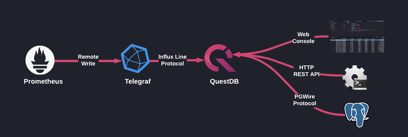
Prometheus is a common time series database that is already installed in many Kubernetes clusters. We will be leveraging its remote write functionality to pipe data into QuestDB for querying and storage. However, since Prometheus remote write does not support the QuestDB-recommended InfluxDB Line Protocol (ILP) as a serialization format, we need to use a proxy to translate Prometheus-formatted metrics into ILP messages. We will be use Influx Data's Telegraf as this translation component.
Now, with our data in QuestDB, we can use SQL to query our metrics using any one of the supported methods: the Web Console, PostgreSQL wire protocol, or HTTP REST API.
Here's a quick overview of the architecture:
Prometheus remote write
While Prometheus operates on an interval-based pull model, it also has the ability to push metrics to remote sources. This is known as "remote write" capability, and is easily configurable in a yaml file. Here's an example of a basic remote write configuration:
remoteWrite:
  - url: http://default.telegraf.svc:9999/write
    name: questdb-telegraf
    remote_timeout: 10s
This yaml will configure Prometheus to send samples to the specified url with a 10 second timeout. In this case, we will be forwarding our metrics on to telegraf, with a custom port and endpoint that we can specify in the telegraf config (see below for more details). There are also a variety of other remote write options, allowing users to customize timeouts, headers, authentication, and additional relabling configs before writing to the remote data store. All of the possible options can be found on the Prometheus website.
QuestDB ILP and Telegraf
Now that we have our remote write configured, we need to set up its destination.
Installing telegraf into a cluster is straightforward, just helm install its
Helm chart.
We do need to configure telegraf to read from a web socket (where Prometheus is configured to writing to) and send to QuestDB for long-term storage. In a Kubernetes deployment, these options can be set in the config section of the telegraf Helm chart's values.yaml file.
Input Configuration
Since telegraf will be receiving metrics from Prometheus, we need to open a port that enables communication between the two services. Telegraf has an HTTP listener plugin that allows it to listen for traffic on a specified port. We also need to configure the path of the listener to match our Promtheus remote write url.
The HTTP listener (v2) supports multiple data formats to consume via its plugin architecture. A full list of options can be found in the telegraf docs. We will be using the Prometheus Remote Write Parser Plugin to accept our Prometheus messages.
Here is how this setup looks in the telegraf config:
[[inputs.http_listener_v2]]
  ## Address and port to host HTTP listener on
  service_address = ":9999"

  ## Paths to listen to.
  paths = ["/write"]

  ## Data format to consume.
  data_format = "prometheusremotewrite"
When passing these values to the Helm chart, you can use this yaml
specification:
config:
  inputs:
    - http_listener_v2:
        service_address: ":9999"
        path: "/write"
        data_format: prometheusremotewrite
Output configuration
We recommend that you use the
InfluxDB Line Protocol
(ILP) over TCP to insert data into QuestDB. Luckily, telegraf includes an ILP
output plugin! But unfortunately, this is not a plug-and-play solution. By
default, all metrics will be written to a single measurement,
prometheus_remote_write, with the individual metric's key being sent over the
wire as a field. In practice, this means that all of your metrics will be
written to a single QuestDB table, called prometheus_remote_write. There will
then be an additional column for every single metric AND field that you are
capturing. This leads to a large table, with potentially thousands of columns,
that's difficult to work with and contains all sparse data, which could
negatively impact performance.
To fix this problem, Telegraf provides us with a sample starlark script that transforms each measurement such that we will have a table-per-metric in QuestDB. This script will run for every metric that telegraf receives, so the output will be formatted correctly.
This is what telegraf's output config looks like:
[[outputs.socket_writer]]
  ## Address and port to write to
  address = "tcp://questdb.questdb.svc:9009"

[[processors.starlark]]
      source = '''
    def apply(metric):
      if metric.name == "prometheus_remote_write":
            for k, v in metric.fields.items():
                metric.name = k
                metric.fields["value"] = v
                metric.fields.pop(k)
      return metric
    '''
As an added benefit to using ILP with QuestDB, we don't even have to worry about
each metric's fieldset. Over ILP, QuestDB
automatically creates tables
for new metrics. It also adds new columns for fields that it hasn't seen before,
and INSERTs nulls for any missing fields.
Helm configuration
I've found that the easiest way to configure the values.yaml file is to mount
the starlark script as a volume, and add a reference to it in the config. This
way we don't need to deal with any whitespace-handling or special indentation in
our ConfigMap specification.
The output and starlark Helm configuration would look like this:
# continued from above
# config:
outputs:
  - socket_writer:
      address: tcp://questdb.questdb.svc:9009
processors:
  - starlark:
      script: /opt/telegraf/remotewrite.star
We also need to add the volume and mount at the root level of the values.yaml:
volumes:
  - name: starlark-script
    configMap:
      name: starlark-script
mountPoints:
  - name: starlark-script
    mountPath: /opt/telegraf
    subpath: remotewrite.star
This volume references a ConfigMap that contains the starlark script from the above example:
---
apiVersion: v1
kind: ConfigMap
metadata:
  name: starlark-script
data:
  remotewrite.star: |
    def apply(metric):
      ...
Querying metrics with SQL
QuestDB has some powerful SQL extensions that can simplify writing time series queries. For example, given the standard set of metrics that a typical Prometheus installation collects, we can use QuestDB to not only find pods with the highest memory usage in a cluster (over a 6 month period), but also find the specific time period when the memory usage spiked. We can even access custom labels to help identify the pods with a human-readable name (instead of the long alphanumeric name assigned to pods by deployments or stateful sets). This is all performed with a simple SQL syntax using JOINs (enhanced by the ASOF keyword) and SAMPLE BY to bucket data into days with a simple line of SQL:
SELECT l.custom_label, w.timestamp, max(w.value / r.value) as mem_usage
FROM container_memory_working_set_bytes AS w
ASOF JOIN kube_pod_labels AS l ON (w.pod = l.pod)
ASOF JOIN kube_pod_container_resource_limits AS r ON (
  r.pod = w.pod AND
  r.container = w.container
)
WHERE custom_label IS NOT NULL
  AND r.resource = 'memory'
  AND w.timestamp > '2022-06-01'
SAMPLE BY 1d
ALIGN TO CALENDAR TIME ZONE 'Europe/Berlin'
ORDER BY mem_usage DESC;
Here's a sample output of that query:
| custom_label | timestamp | mem_usage |
|---|---|---|
| keen austin | 2022-07-04T16:18:00.000000Z | 0.999853875401 |
| optimistic banzai | 2022-07-12T16:18:00.000000Z | 0.9763028946 |
| compassionate taussig | 2022-07-11T16:18:00.000000Z | 0.975367909527 |
| cranky leakey | 2022-07-11T16:18:00.000000Z | 0.974941994418 |
| quirky morse | 2022-07-05T16:18:00.000000Z | 0.95084235665 |
| admiring panini | 2022-06-21T16:18:00.000000Z | 0.925567626953 |
This is only one of many ways that you can use QuestDB to write powerful time-series queries that you can use for one-off investigation or to power dashboards.
Metric retention
Since databases storing infrastructure metrics can grow to extreme sizes over
time, it is important to enforce a retention period to free up space by deleting
old metrics. Even though QuestDB does not support the traditional DELETE SQL
command, you can still implement metric retention by using the DROP PARTITION
command.
In QuestDB, data is stored by columns on-disk and optionally partitioned by a
time duration. By default, when using ILP to ingest metrics, and a new table is
automatically created, it is partitioned by DAY. This allows us to
DROP PARTITIONs on a daily basis. If you need a different partitioning scheme,
you can create the table with your desired partition period before ingesting any
data over ILP, since ALTER TABLE does not support any changes to table
partitioning. But since ILP does automatically add columns, the table
specification can be very simple, with just the name and a timestamp column.
Once you've decided on your desired metric retention period, you can create a cron job that removes all partitions older than your oldest retention date. This will help keep your storage usage in check.
For more information about data retention in QuestDB, you can check out the docs.
Working example
I have created a working example of this setup in a repo, sklarsa/questdb-metrics-blog-post. The entire example runs in a local Kind cluster.
To run the example, execute the following commands:
git clone https://github.com/sklarsa/questdb-metrics-blog-post.git
cd questdb-metrics-blog-post
./run.sh
After a few minutes, all pods should be in ready with the following prompt:
You can now access QuestDB here: http://localhost:9000
Ctrl-C to exit
Forwarding from 127.0.0.1:9000 -> 9000
Forwarding from [::1]:9000 -> 9000
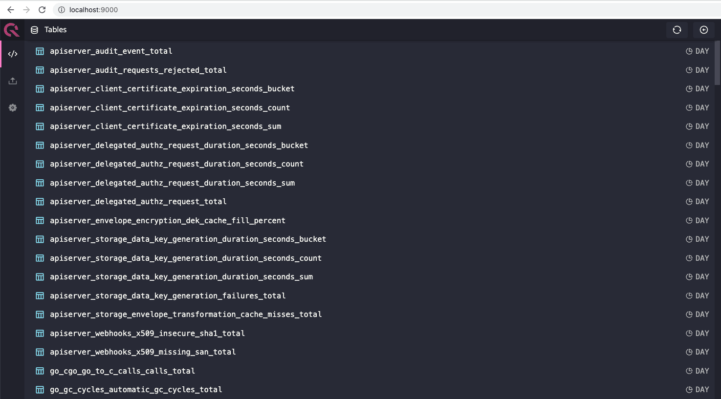
From here, you can navigate to http://localhost:9000 and explore the metrics that are being ingested into QuestDB. The default Prometheus scrape interval is 30 seconds, so there might not be a ton of data in there, but you should see a list of tables, one per each metric that we are collecting:
Once you're done, you can clean up the entire experiment by deleting the cluster:
./cleanup.sh
Conclusion
QuestDB can be a very powerful piece in the Cloud Engineer's toolkit. It grants you the ability to run complex time-series queries across multiple metrics with unparalleled speed in the world's most ubiquitous query language, SQL. Every second counts when debugging an outage at 2AM, and reducing the cognitive load of writing queries, as well as their execution time, is a game-changer for me.